快速入门教程
GluonTS 包含
- 许多预构建模型
- 用于构建新模型的组件(似然函数、特征处理管道、日历特征等)
- 数据加载和处理
- 绘图和评估工具
- 人工和真实数据集(仅限具有许可的外部数据集)
%matplotlib inline
import numpy as np
import pandas as pd
import matplotlib.pyplot as plt
import json
from pathlib import Path
环境说明
注意我们采取新版的GluonTS。安装其之前,确保安装好如下版本的torch系列包,防止后续出现版本不兼容问题:
pip install torch==2.1.0 torchvision==0.16.0 torchaudio==2.1.0 --index-url https://download.pytorch.org/whl/cu118安装GluonTS torch版本:
pip install "gluonts[torch]==0.14.4"数据集
提供的预设数据集
GluonTS 附带了许多公开可用的数据集。
from gluonts.dataset.repository.datasets import get_dataset, dataset_names
from gluonts.dataset.util import to_pandas注意旧版写法为from gluonts.dataset.repository import get_dataset, dataset_names,新版中已不再适用。
print(f"Available datasets: {dataset_names}")
'''
output:
Available datasets: ['constant', 'exchange_rate', 'solar-energy', 'electricity', 'traffic', 'exchange_rate_nips', 'electricity_nips', 'traffic_nips', 'solar_nips', 'wiki2000_nips', 'wiki-rolling_nips', 'taxi_30min', 'kaggle_web_traffic_with_missing', 'kaggle_web_traffic_without_missing', 'kaggle_web_traffic_weekly', 'm1_yearly', 'm1_quarterly', 'm1_monthly', 'nn5_daily_with_missing', 'nn5_daily_without_missing', 'nn5_weekly', 'tourism_monthly', 'tourism_quarterly', 'tourism_yearly', 'cif_2016', 'london_smart_meters_without_missing', 'wind_farms_without_missing', 'car_parts_without_missing', 'dominick', 'fred_md', 'pedestrian_counts', 'hospital', 'covid_deaths', 'kdd_cup_2018_without_missing', 'weather', 'm3_monthly', 'm3_quarterly', 'm3_yearly', 'm3_other', 'm4_hourly', 'm4_daily', 'm4_weekly', 'm4_monthly', 'm4_quarterly', 'm4_yearly', 'm5', 'uber_tlc_daily', 'uber_tlc_hourly', 'airpassengers', 'australian_electricity_demand', 'electricity_hourly', 'electricity_weekly', 'rideshare_without_missing', 'saugeenday', 'solar_10_minutes', 'solar_weekly', 'sunspot_without_missing', 'temperature_rain_without_missing', 'vehicle_trips_without_missing']
'''
要下载内置数据集之一,只需使用上述名称之一调用 get_dataset。GluonTS 可以重新使用已保存的数据集,这样下次就不需要再次下载。
有时候,在linux服务器上调用get_dataset时,可能会遇到http连接超时的报错,这是因为访问外网受限。建议在本地挂梯子调用这句话,然后将下载好的完整数据集文件夹上传至服务器中。注意下面我们额外强调了path参数,显式指定了数据集下载保存路径,否则它会默认下载到/home/你的用户名/.mxnet/下。
dataset = get_dataset("m4_hourly", path=Path("./datasets"))通常,GluonTS 提供的数据集是由三个主要成员组成的对象:
dataset.train是一个可迭代的数据项集合,用于训练。每个数据项对应一个时间序列。dataset.test是一个可迭代的数据项集合,用于推理。测试数据集是训练数据集的扩展版本,其中包含每个时间序列末尾在训练期间未见的窗口。此窗口的长度等于推荐的预测长度。dataset.metadata包含数据集的元数据,例如时间序列的频率、推荐的预测范围、相关特征等。
entry = next(iter(dataset.train))
train_series = to_pandas(entry)
train_series.plot()
plt.grid(which="both")
plt.legend(["train series"], loc="upper left")
plt.show()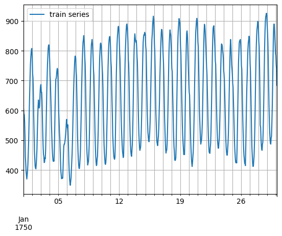
entry = next(iter(dataset.test))
test_series = to_pandas(entry)
test_series.plot()
plt.axvline(train_series.index[-1], color="r")  # end of train dataset
plt.grid(which="both")
plt.legend(["test series", "end of train series"], loc="upper left")
plt.show()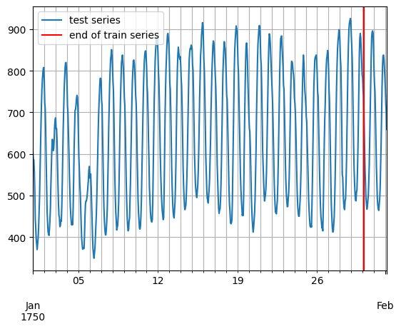
print(
    f"Length of forecasting window in test dataset: {len(test_series) - len(train_series)}"
)
print(f"Recommended prediction horizon: {dataset.metadata.prediction_length}")
print(f"Frequency of the time series: {dataset.metadata.freq}")
'''
output:
Length of forecasting window in test dataset: 48
Recommended prediction horizon: 48
Frequency of the time series: H
'''
自定义数据集
在此需要强调,GluonTS 对用户自定义数据集的格式没有严格要求。自定义数据集唯一的要求是可迭代,并包含“target”和“start”字段。为了更清楚地说明这一点,假设常见的情况是数据集采用 numpy.array 的形式,并且时间序列的索引采用 pandas.Period(每个时间序列可能不同)。
N = 10  # number of time series
T = 100  # number of timesteps
prediction_length = 24
freq = "1H"
custom_dataset = np.random.normal(size=(N, T))
start = pd.Period("01-01-2019", freq=freq)  # can be different for each time series
现在,您只需两行代码即可分割数据集并将其转换为适合 GluonTS 的格式
from gluonts.dataset.common import ListDataset

# train dataset: cut the last window of length "prediction_length", add "target" and "start" fields
train_ds = ListDataset(
    [{"target": x, "start": start} for x in custom_dataset[:, :-prediction_length]],
    freq=freq,
)
# test dataset: use the whole dataset, add "target" and "start" fields
test_ds = ListDataset(
    [{"target": x, "start": start} for x in custom_dataset], freq=freq
)训练现有模型(Estimator)
GluonTS 附带了许多预构建模型。用户只需配置一些超参数。现有模型主要侧重于(但不限于)概率预测。概率预测是以概率分布形式进行的预测,而不仅仅是单一的点估计。
我们将从 GluonTS 预构建的前馈神经网络估计器开始,这是一个简单但功能强大的预测模型。我们将使用该模型来演示模型训练、生成预测和评估结果的过程。
GluonTS 内置的前馈神经网络(SimpleFeedForwardEstimator)接受长度为 context_length 的输入窗口,并预测后续 prediction_length 个值的分布。在 GluonTS 的术语中,前馈神经网络模型是 Estimator 的一个示例。在 GluonTS 中,Estimator 对象代表一个预测模型以及其系数、权重等详细信息。
通常,每个估计器(预构建或自定义)都通过许多超参数进行配置,这些超参数可以是所有估计器通用的(但不强制要求),例如 prediction_length,也可以是特定于该估计器的,例如神经网络的层数或 CNN 的步长。下面我们导入torch版本的估计器。
from gluonts.torch import SimpleFeedForwardEstimator在旧版本中,每个估计器都由一个 Trainer 进行配置,Trainer 定义了模型如何训练,例如 epoch 数量、学习率等,要额外注意,在当前的新版本中此写法已不受支持。我们直接在Estimator对象的字典型参数trainer_kwargs中配置训练参数。
estimator = SimpleFeedForwardEstimator(
    hidden_dimensions=[10],
    prediction_length=dataset.metadata.prediction_length,
    context_length=100,
    trainer_kwargs={
        "max_epochs": 5,
        "accelerator": "gpu",
        "devices": 1,
    }
)
在指定了所有必需的超参数来配置我们的估计器后,我们可以使用训练数据集 dataset.train 调用估计器的 train 方法来训练它。训练算法返回一个拟合好的模型(在 GluonTS 术语中称为 Predictor),该模型可用于生成预测。
predictor = estimator.train(dataset.train)可视化和评估预测
有了预测器后,我们现在可以预测 dataset.test 的最后一个窗口并评估模型的性能。
GluonTS 附带了 make_evaluation_predictions 函数,该函数可以自动化预测和模型评估过程。大致来说,此函数执行以下步骤:
- 移除我们想要预测的
dataset.test中长度为prediction_length的最后一个窗口 - 估计器使用剩余数据来预测刚刚移除的“未来”窗口(以样本路径的形式)
- 该模块输出预测样本路径和
dataset.test(作为 Python 生成器对象)
from gluonts.evaluation import make_evaluation_predictions

forecast_it, ts_it = make_evaluation_predictions(
    dataset=dataset.test,  # test dataset
    predictor=predictor,  # predictor
    num_samples=100,  # number of sample paths we want for evaluation
)
首先,我们可以将这些生成器转换为列表,以便后续计算。
forecasts = list(forecast_it)
tss = list(ts_it)
我们可以检查这些列表的第一个元素(对应于数据集的第一个时间序列)。让我们从包含时间序列的列表 tss 开始。我们期望 tss 的第一个条目包含 dataset.test 的第一个时间序列的(目标值)。如下代码可以验证这两者是相同的。
# first entry of the time series list
ts_entry = tss[0]
# first 5 values of the time series (convert from pandas to numpy)
np.array(ts_entry[:5]).reshape(
    -1,
)
# output: array([605., 586., 586., 559., 511.], dtype=float32)
# first entry of dataset.test
dataset_test_entry = next(iter(dataset.test))
# first 5 values
dataset_test_entry["target"][:5]
# output: array([605., 586., 586., 559., 511.], dtype=float32)
forecast 列表中的条目稍微复杂一些。它们是包含所有样本路径的对象,样本路径的形式是维度为 (num_samples, prediction_length) 的 numpy.ndarray,还包含预测的开始日期、时间序列的频率等。只需调用预测对象的相应属性即可访问所有这些信息。
# first entry of the forecast list
forecast_entry = forecasts[0]
注意如下新版本的predictor输出结果的代码:
print(f"Distribution of the forecast samples: {forecast_entry.distribution}")
samples = forecast_entry.distribution.sample((100,)) # 新版本写法:从预测的分布中采样100条路径
print(f"Dimension of samples: {samples.shape}")
print(f"Start date of the forecast window: {forecast_entry.start_date}")
print(f"Frequency of the time series: {forecast_entry.freq}")
我们还可以进行计算来汇总样本路径,例如计算预测窗口中每个 48 个时间步长的均值或分位数。
print(f"Mean of the future window:\n {forecast_entry.mean}")
print(f"0.5-quantile (median) of the future window:\n {forecast_entry.quantile(0.5)}")

'''
output:
Mean of the future window:
 [601.62616 571.62506 478.83017 449.07114 442.25357 475.66016 458.40277
 487.0524  489.93985 560.6161  593.5261  617.5017  680.78204 703.5066
 776.2343  805.18195 818.439   801.3591  823.86285 824.93445 773.12427
 771.9947  752.93134 674.657   580.7824  584.4749  546.70294 501.74213
 437.55557 466.95404 461.45004 500.73813 505.69696 575.597   588.41644
 611.2112  716.33136 778.6789  787.3356  855.0106  842.9774  841.0472
 851.654   842.5805  836.80914 788.31415 771.4369  697.8607 ]
0.5-quantile (median) of the future window:
 [601.62616 571.62506 478.83017 449.07114 442.25357 475.66016 458.40277
 487.0524  489.93985 560.6161  593.5261  617.5017  680.78204 703.5066
 776.2343  805.18195 818.439   801.3591  823.86285 824.93445 773.12427
 771.9947  752.93134 674.657   580.7824  584.4749  546.70294 501.74213
 437.55557 466.95404 461.45004 500.73813 505.69696 575.597   588.41644
 611.2112  716.33136 778.6789  787.3356  855.0106  842.9774  841.0472
 851.654   842.5805  836.80914 788.31415 771.4369  697.8607 ]
'''
Forecast 对象有一个 plot 方法,可以将预测路径汇总为均值、预测区间等。预测区间以不同的颜色阴影表示,形成“扇形图”。
plt.plot(ts_entry[-150:].to_timestamp())
forecast_entry.plot(show_label=True)
plt.legend()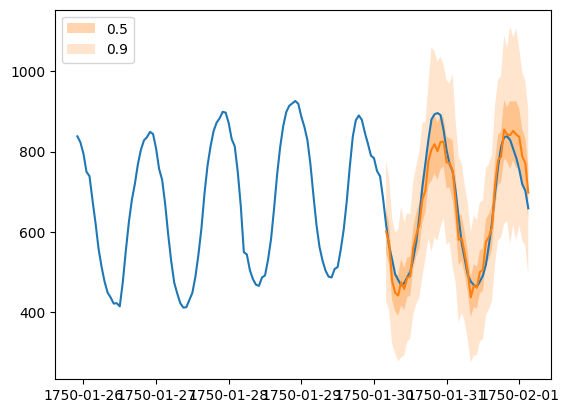
我们还可以从数值上评估预测的质量。在 GluonTS 中,Evaluator 类可以计算聚合性能指标,以及每个时间序列的指标(这对于分析跨异构时间序列的性能非常有用)。
from gluonts.evaluation import Evaluator
evaluator = Evaluator(quantiles=[0.1, 0.5, 0.9])
agg_metrics, item_metrics = evaluator(tss, forecasts)
聚合指标 agg_metrics 聚合了跨时间步长和跨时间序列的性能。
print(json.dumps(agg_metrics, indent=4)){
"MSE": 10330287.941363767,
"abs_error": 9888776.191505432,
"abs_target_sum": 145558863.59960938,
"abs_target_mean": 7324.822041043146,
"seasonal_error": 336.9046924038305,
"MASE": 3.298529737437924,
"MAPE": 0.24230639967653486,
"sMAPE": 0.1844004778050474,
"MSIS": 64.15294911907903,
"num_masked_target_values": 0.0,
"QuantileLoss[0.1]": 4685229.677179908,
"Coverage[0.1]": 0.10487117552334944,
"QuantileLoss[0.5]": 9888776.174993515,
"Coverage[0.5]": 0.5401066827697263,
"QuantileLoss[0.9]": 7182032.328086851,
"Coverage[0.9]": 0.8878824476650563,
"RMSE": 3214.076530103751,
"NRMSE": 0.4387924392011613,
"ND": 0.06793661304409888,
"wQuantileLoss[0.1]": 0.032187869301230805,
"wQuantileLoss[0.5]": 0.0679366129306608,
"wQuantileLoss[0.9]": 0.04934108545833773,
"mean_absolute_QuantileLoss": 7252012.726753425,
"mean_wQuantileLoss": 0.049821855896743115,
"MAE_Coverage": 0.39596081588835214,
"OWA": NaN
}需要额外注意这里的mean_wQuantileLoss指标,它实际上是论文中常用指标CRPS的近似替代。当然为了使其更加近似、精确,可以在Evaluator的参数quantiles多设置一些分位数:
evaluator = Evaluator(
    quantiles=[i / 100.0 for i in range(1, 100)]
)

agg_metrics, item_metrics = evaluator(tss, forecasts)
个别指标仅聚合跨时间步长的性能。
item_metrics.head()输出表格:
| item_id | forecast_start | MSE | abs_error | abs_target_sum | abs_target_mean | seasonal_error | MASE | MAPE | sMAPE | num_masked_target_values | ND | MSIS | QuantileLoss[0.1] | Coverage[0.1] | QuantileLoss[0.5] | Coverage[0.5] | QuantileLoss[0.9] | Coverage[0.9] | |
|---|---|---|---|---|---|---|---|---|---|---|---|---|---|---|---|---|---|---|---|
| 0 | 0 | 1750-01-30 04:00 | 3309.237305 | 2154.689453 | 31644.0 | 659.250000 | 42.371302 | 1.059428 | 0.067252 | 0.064834 | 0.0 | 0.068092 | 13.231213 | 935.300177 | 0.041667 | 2154.689484 | 0.708333 | 1459.305225 | 1.000000 |
| 1 | 1 | 1750-01-30 04:00 | 182585.895833 | 18652.218750 | 124149.0 | 2586.437500 | 165.107988 | 2.353538 | 0.159426 | 0.146121 | 0.0 | 0.150241 | 14.012219 | 4414.383215 | 0.270833 | 18652.218994 | 0.979167 | 8807.242969 | 1.000000 |
| 2 | 2 | 1750-01-30 04:00 | 31560.596354 | 6341.560547 | 65030.0 | 1354.791667 | 78.889053 | 1.674704 | 0.087524 | 0.093271 | 0.0 | 0.097517 | 13.391114 | 3399.184241 | 0.000000 | 6341.560669 | 0.208333 | 2718.548511 | 0.729167 |
| 3 | 3 | 1750-01-30 04:00 | 161919.552083 | 15676.248047 | 235783.0 | 4912.145833 | 258.982249 | 1.261046 | 0.065586 | 0.064962 | 0.0 | 0.066486 | 14.689635 | 8973.606250 | 0.062500 | 15676.248291 | 0.437500 | 8183.246777 | 1.000000 |
| 4 | 4 | 1750-01-30 04:00 | 104537.510417 | 11086.554688 | 131088.0 | 2731.000000 | 200.494083 | 1.152004 | 0.085404 | 0.079762 | 0.0 | 0.084573 | 12.690474 | 4597.160254 | 0.083333 | 11086.554077 | 0.791667 | 7307.160693 | 1.000000 |
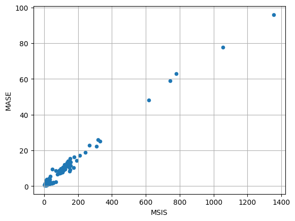
绘制一份MASE-MSIS散点图像:
item_metrics.plot(x="MSIS", y="MASE", kind="scatter")
plt.grid(which="both")
plt.show()